probability

    li f e sa v e r

    All the tools you need to understand chance

    Steven J. Miller

    PRINCETON UNIVERSITY PRESS

    Princeton and OxfordCopyright c 2017 by Princeton University Press

    Published by Princeton University Press, 41 William Street,Princeton, New Jersey 08540

    In the United Kingdom: Princeton University Press, 6 Oxford Street,Woodstock, Oxfordshire OX20 1TR

    press.princeton.edu

    Names: Miller, Steven J., 1974–

    Title: The probability lifesaver : all the tools you need to understand

    chance Steven J. Miller.

    Description: Princeton : Princeton University Press, [2017] | Series: A

    Princeton lifesaver study guide | Includes bibliographical references and index.

    Identi?ers: LCCN 2016040785| ISBN 9780691149547 (hardcover : alk. paper) |

    ISBN 9780691149554 (pbk. : alk. paper)

    Subjects: LCSH: Probabilities. | Chance. | Games of chance (Mathematics) |

    Random variables.

    Classi?cation: LCC QA273 .M55185 2017 | DDC 519.2-dc23 LC record

    available at https:lccn.loc.gov2016040785

    British Library Cataloging-in-Publication Data is available

    This book has been composed in Times New Roman with Stencil and Avant Garde

    Typeset by Nova Techset Pvt Ltd, Bangalore, India

    Printed in the United States of America

    Library of Congress Cataloging-in-Publication DataContents

    Note to Readers xv

    How to Use This Book xix

    I General Theory 1

    1 Introduction 3

    1.1 Birthday Problem 4

    1.1.1 Stating the Problem 4

    1.1.2 Solving the Problem 6

    1.1.3 Generalizing the Problem and Solution: Ef?ciencies 11

    1.1.4 Numerical Test 14

    1.2 From Shooting Hoops to the Geometric Series 16

    1.2.1 The Problem and Its Solution 16

    1.2.2 Related Problems 21

    1.2.3 General Problem Solving Tips 25

    1.3 Gambling 27

    1.3.1 The 2008 Super Bowl Wager 28

    1.3.2 Expected Returns 28

    1.3.3 The Value of Hedging 29

    1.3.4 Consequences 31

    1.4 Summary 31

    1.5 Exercises 34

    2 Basic Probability Laws 40

    2.1 Paradoxes 41

    2.2 Set Theory Review 43

    2.2.1 Coding Digression 47

    2.2.2 Sizes of In?nity and Probabilities 48

    2.2.3 Open and Closed Sets 50

    2.3 Outcome Spaces, Events, and the Axioms of Probability 52

    2.4 Axioms of Probability 57

    2.5 Basic Probability Rules 59

    2.5.1 Law of Total Probability 60

    2.5.2 Probabilities of Unions 61

    2.5.3 Probabilities of Inclusions 64

    2.6 Probability Spaces and σ-algebras 652.7 Appendix: Experimentally Finding Formulas 70

    2.7.1 Product Rule for Derivatives 71

    2.7.2 Probability of a Union 72

    2.8 Summary 73

    2.9 Exercises 73

    3 Counting I: Cards 78

    3.1 Factorials and Binomial Coef?cients 79

    3.1.1 The Factorial Function 79

    3.1.2 Binomial Coef?cients 82

    3.1.3 Summary 87

    3.2 Poker 88

    3.2.1 Rules 88

    3.2.2 Nothing 90

    3.2.3 Pair 92

    3.2.4 Two Pair 95

    3.2.5 Three of a Kind 96

    3.2.6 Straights, Flushes, and Straight Flushes 96

    3.2.7 Full House and Four of a Kind 97

    3.2.8 Practice Poker Hand: I 98

    3.2.9 Practice Poker Hand: II 100

    3.3 Solitaire 101

    3.3.1 Klondike 102

    3.3.2 Aces Up 105

    3.3.3 FreeCell 107

    3.4 Bridge 108

    3.4.1 Tic-tac-toe 109

    3.4.2 Number of Bridge Deals 111

    3.4.3 Trump Splits 117

    3.5 Appendix: Coding to Compute Probabilities 120

    3.5.1 Trump Split and Code 120

    3.5.2 Poker Hand Codes 121

    3.6 Summary 124

    3.7 Exercises 124

    4 Conditional Probability, Independence, and

    Bayes’ Theorem 128

    4.1 Conditional Probabilities 129

    4.1.1 Guessing the Conditional Probability Formula 131

    4.1.2 Expected Counts Approach 132

    4.1.3 Venn Diagram Approach 133

    4.1.4 The Monty Hall Problem 135

    4.2 The General Multiplication Rule 136

    4.2.1 Statement 136

    4.2.2 Poker Example 136

    4.2.3 Hat Problem and Error Correcting Codes 138

    4.2.4 Advanced Remark: De?nition of Conditional Probability 138

    4.3 Independence 139

    4.4 Bayes’ Theorem 1424.5 Partitions and the Law of Total Probability 147

    4.6 Bayes’ Theorem Revisited 150

    4.7 Summary 151

    4.8 Exercises 152

    5 Counting II: Inclusion-Exclusion 156

    5.1 Factorial and Binomial Problems 157

    5.1.1 “How many” versus “What’s the probability” 157

    5.1.2 Choosing Groups 159

    5.1.3 Circular Orderings 160

    5.1.4 Choosing Ensembles 162

    5.2 The Method of Inclusion-Exclusion 163

    5.2.1 Special Cases of the Inclusion-Exclusion Principle 164

    5.2.2 Statement of the Inclusion-Exclusion Principle 167

    5.2.3 Justi?cation of the Inclusion-Exclusion Formula 168

    5.2.4 Using Inclusion-Exclusion: Suited Hand 171

    5.2.5 The At Least to Exactly Method 173

    5.3 Derangements 176

    5.3.1 Counting Derangements 176

    5.3.2 The Probability of a Derangement 178

    5.3.3 Coding Derangement Experiments 178

    5.3.4 Applications of Derangements 179

    5.4 Summary 181

    5.5 Exercises 182

    6 Counting III: Advanced Combinatorics 186

    6.1 Basic Counting 187

    6.1.1 Enumerating Cases: I 187

    6.1.2 Enumerating Cases: II 188

    6.1.3 Sampling With and Without Replacement 192

    6.2 Word Orderings 199

    6.2.1 Counting Orderings 200

    6.2.2 Multinomial Coef?cients 202

    6.3 Partitions 205

    6.3.1 The Cookie Problem 205

    6.3.2 Lotteries 207

    6.3.3 Additional Partitions 212

    6.4 Summary 214

    6.5 Exercises 215

    II Introduction to Random Variables 219

    7 Introduction to Discrete Random Variables 221

    7.1 Discrete Random Variables: De?nition 221

    7.2 Discrete Random Variables: PDFs 223

    7.3 Discrete Random Variables: CDFs 2267.4 Summary 233

    7.5 Exercises 235

    8 Introduction to Continuous Random Variables 238

    8.1 Fundamental Theorem of Calculus 239

    8.2 PDFs and CDFs: De?nitions 241

    8.3 PDFs and CDFs: Examples 243

    8.4 Probabilities of Singleton Events 248

    8.5 Summary 250

    8.6 Exercises 250

    9 Tools: Expectation 254

    9.1 Calculus Motivation 255

    9.2 Expected Values and Moments 257

    9.3 Mean and Variance 261

    9.4 Joint Distributions 265

    9.5 Linearity of Expectation 269

    9.6 Properties of the Mean and the Variance 274

    9.7 Skewness and Kurtosis 279

    9.8 Covariances 280

    9.9 Summary 281

    9.10 Exercises 281

    10 Tools: Convolutions and Changing Variables 285

    10.1 Convolutions: De?nitions and Properties 286

    10.2 Convolutions: Die Example 289

    10.2.1 Theoretical Calculation 289

    10.2.2 Convolution Code 290

    10.3 Convolutions of Several Variables 291

    10.4 Change of Variable Formula: Statement 294

    10.5 Change of Variables Formula: Proof 297

    10.6 Appendix: Products and Quotients

    of Random Variables 302

    10.6.1 Density of a Product 302

    10.6.2 Density of a Quotient 303

    10.6.3 Example: Quotient of Exponentials 304

    10.7 Summary 305

    10.8 Exercises 305

    11 Tools: Differentiating Identities 309

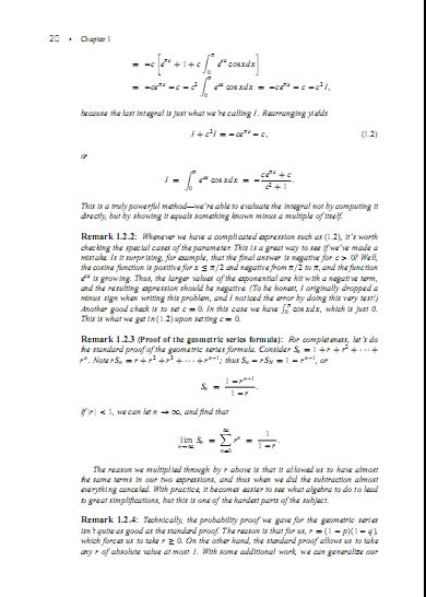
    11.1 Geometric Series Example 310

    11.2 Method of Differentiating Identities 313

    11.3 Applications to Binomial Random Variables 314

    11.4 Applications to Normal Random Variables 31711.5 Applications to Exponential

    Random Variables 320

    11.6 Summary 322

    11.7 Exercises 323

    III Special Distributions 325

    12 Discrete Distributions 327

    12.1 The Bernoulli Distribution 328

    12.2 The Binomial Distribution 328

    12.3 The Multinomial Distribution 332

    12.4 The Geometric Distribution 335

    12.5 The Negative Binomial Distribution 336

    12.6 The Poisson Distribution 340

    12.7 The Discrete Uniform Distribution 343

    12.8 Exercises 346

    13 Continuous Random Variables:

    Uniform and Exponential 349

    13.1 The Uniform Distribution 349

    13.1.1 Mean and Variance 350

    13.1.2 Sums of Uniform Random Variables 352

    13.1.3 Examples 354

    13.1.4 Generating Random Numbers Uniformly 356

    13.2 The Exponential Distribution 357

    13.2.1 Mean and Variance 357

    13.2.2 Sums of Exponential Random Variables 361

    13.2.3 Examples and Applications of Exponential Random

    Variables 364

    13.2.4 Generating Random Numbers from

    Exponential Distributions 365

    13.3 Exercises 367

    14 Continuous Random Variables: The Normal Distribution 371

    14.1 Determining the Normalization Constant 372

    14.2 Mean and Variance 375

    14.3 Sums of Normal Random Variables 379

    14.3.1 Case 1: μX = μY = 0and σ2

    X = σ2

    Y = 1 380

    14.3.2 Case 2: General μX ,μY and σ2

    X ,σ2

    Y 383

    14.3.3 Sums of Two Normals: Faster Algebra 385

    14.4 Generating Random Numbers from

    Normal Distributions 386

    14.5 Examples and the Central Limit Theorem 392

    14.6 Exercises 39315 The Gamma Function and Related Distributions 398

    15.1 Existence of  (s) 398

    15.2 The Functional Equation of  (s) 400

    15.3 The Factorial Function and  (s) 404

    15.4 Special Values of  (s) 405

    15.5 The Beta Function and the Gamma Function 407

    15.5.1 Proof of the Fundamental Relation 408

    15.5.2 The Fundamental Relation and (12) 410

    15.6 The Normal Distribution and the Gamma Function 411

    15.7 Families of Random Variables 412

    15.8 Appendix: Cosecant Identity Proofs 413

    15.8.1 The Cosecant Identity: First Proof 414

    15.8.2 The Cosecant Identity: Second Proof 418

    15.8.3 The Cosecant Identity: Special Case s=12 421

    15.9 Cauchy Distribution 423

    15.10 Exercises 424

    16 The Chi-square Distribution 427

    16.1 Origin of the Chi-square Distribution 429

    16.2 Mean and Variance of X ～χ2

    (1) 430

    16.3 Chi-square Distributions and Sums of Normal Random

    Variables 432

    16.3.1 Sums of Squares by Direct Integration 434

    16.3.2 Sums of Squares by the Change of Variables Theorem 434

    16.3.3 Sums of Squares by Convolution 439

    16.3.4 Sums of Chi-square Random Variables 441

    16.4 Summary 442

    16.5 Exercises 443

    IV Limit Theorems 447

    17 Inequalities and Laws of Large Numbers 449

    17.1 Inequalities 449

    17.2 Markov’s Inequality 451

    17.3 Chebyshev’s Inequality 453

    17.3.1 Statement 453

    17.3.2 Proof 455

    17.3.3 Normal and Uniform Examples 457

    17.3.4 Exponential Example 458

    17.4 The Boole and Bonferroni Inequalities 459

    17.5 Types of Convergence 461

    17.5.1 Convergence in Distribution 461

    17.5.2 Convergence in Probability 463

    17.5.3 Almost Sure and Sure Convergence 463

    17.6 Weak and Strong Laws of Large Numbers 464

    17.7 Exercises 46518 Stirling’s Formula 469

    18.1 Stirling’s Formula and Probabilities 471

    18.2 Stirling’s Formula and Convergence of Series 473

    18.3 From Stirling to the Central Limit Theorem 474

    18.4 Integral Test and the Poor Man’s Stirling 478

    18.5 Elementary Approaches towards

    Stirling’s Formula 482

    18.5.1 Dyadic Decompositions 482

    18.5.2 Lower Bounds towards Stirling: I 484

    18.5.3 Lower Bounds toward Stirling II 486

    18.5.4 Lower Bounds towards Stirling: III 487

    18.6 Stationary Phase and Stirling 488

    18.7 The Central Limit Theorem and Stirling 490

    18.8 Exercises 491

    19 Generating Functions and Convolutions 494

    19.1 Motivation 494

    19.2 De?nition 496

    19.3 Uniqueness and Convergence of

    Generating Functions 501

    19.4 Convolutions I: Discrete Random Variables 503

    19.5 Convolutions II: Continuous Random Variables 507

    19.6 De?nition and Properties of Moment Generating

    Functions 512

    19.7 Applications of Moment Generating Functions 520

    19.8 Exercises 524

    20 Proof of the Central Limit Theorem 527

    20.1 Key Ideas of the Proof 527

    20.2 Statement of the Central Limit Theorem 529

    20.3 Means, Variances, and Standard Deviations 531

    20.4 Standardization 533

    20.5 Needed Moment Generating Function Results 536

    20.6 Special Case: Sums of Poisson

    Random Variables 539

    20.7 Proof of the CLT for General Sums via MGF 542

    20.8 Using the Central Limit Theorem 544

    20.9 The Central Limit Theorem and

    Monte Carlo Integration 545

    20.10 Summary 546

    20.11 Exercises 548

    21 Fourier Analysis and the Central Limit Theorem 553

    21.1 Integral Transforms 554

    21.2 Convolutions and Probability Theory 55821.3 Proof of the Central Limit Theorem 562

    21.4 Summary 565

    21.5 Exercises 565

    V Additional Topics 567

    22 Hypothesis Testing 569

    22.1 Z-tests 570

    22.1.1 Null and Alternative Hypotheses 570

    22.1.2 Signi?cance Levels 571

    22.1.3 Test Statistics 573

    22.1.4 One-sided versus Two-sided Tests 576

    22.2 On p-values 579

    22.2.1 Extraordinary Claims and p-values 580

    22.2.2 Large p-values 580

    22.2.3 Misconceptions about p-values 581

    22.3 On t-tests 583

    22.3.1 Estimating the Sample Variance 583

    22.3.2 From z-tests to t-tests 584

    22.4 Problems with Hypothesis Testing 587

    22.4.1 Type I Errors 587

    22.4.2 Type II Errors 588

    22.4.3 Error Rates and the Justice System 588

    22.4.4 Power 590

    22.4.5 Effect Size 590

    22.5 Chi-square Distributions, Goodness of Fit 590

    22.5.1 Chi-square Distributions and Tests of Variance 591

    22.5.2 Chi-square Distributions and t-distributions 595

    22.5.3 Goodness of Fit for List Data 595

    22.6 Two Sample Tests 598

    22.6.1 Two-sample z-test: Known Variances 598

    22.6.2 Two-sample t-test: Unknown but Same Variances 600

    22.6.3 Unknown and Different Variances 602

    22.7 Summary 604

    22.8 Exercises 605

    23 Difference Equations, Markov Processes,and Probability 607

    23.1 From the Fibonacci Numbers to Roulette 607

    23.1.1 The Double-plus-one Strategy 607

    23.1.2 A Quick Review of the Fibonacci Numbers 609

    23.1.3 Recurrence Relations and Probability 610

    23.1.4 Discussion and Generalizations 612

    23.1.5 Code for Roulette Problem 613

    23.2 General Theory of Recurrence Relations 614

    23.2.1 Notation 614

    23.2.2 The Characteristic Equation 61523.2.3 The Initial Conditions 616

    23.2.4 Proof that Distinct Roots Imply Invertibility 618

    23.3 Markov Processes 620

    23.3.1 Recurrence Relations and Population Dynamics 620

    23.3.2 General Markov Processes 622

    23.4 Summary 622

    23.5 Exercises 623

    24 The Method of Least Squares 625

    24.1 Description of the Problem 625

    24.2 Probability and Statistics Review 626

    24.3 The Method of Least Squares 628

    24.4 Exercises 633

    25 Two Famous Problems and Some Coding 636

    25.1 The MarriageSecretary Problem 636

    25.1.1 Assumptions and Strategy 636

    25.1.2 Probability of Success 638

    25.1.3 Coding the Secretary Problem 641

    25.2 Monty Hall Problem 642

    25.2.1 A Simple Solution 643

    25.2.2 An Extreme Case 644

    25.2.3 Coding the Monty Hall Problem 644

    25.3 Two Random Programs 645

    25.3.1 Sampling with and without Replacement 645

    25.3.2 Expectation 646

    25.4 Exercises 646

    Appendix A Proof Techniques 649

    A.1 How to Read a Proof 650

    A.2 Proofs by Induction 651

    A.2.1 Sums of Integers 653

    A.2.2 Divisibility 655

    A.2.3 The Binomial Theorem 656

    A.2.4 Fibonacci Numbers Modulo 2 657

    A.2.5 False Proofs by Induction 659

    A.3 Proof by Grouping 660

    A.4 Proof by Exploiting Symmetries 661

    A.5 Proof by Brute Force 663

    A.6 Proof by Comparison or Story 664

    A.7 Proof by Contradiction 666

    A.8 Proof by Exhaustion (or Divide and Conquer) 668

    A.9 Proof by Counterexample 669

    A.10 Proof by Generalizing Example 669

    A.11 Dirichlet’s Pigeon-Hole Principle 670

    A.12 Proof by Adding Zero or Multiplying by One 671Appendix B Analysis Results 675

    B.1 The Intermediate and Mean Value Theorems 675

    B.2 Interchanging Limits, Derivatives, and Integrals 678

    B.2.1 Interchanging Orders: Theorems 678

    B.2.2 Interchanging Orders: Examples 679

    B.3 Convergence Tests for Series 682

    B.4 Big-Oh Notation 685

    B.5 The Exponential Function 688

    B.6 Proof of the Cauchy-Schwarz Inequality 691

    B.7 Exercises 692

    Appendix C Countable and Uncountable Sets 693

    C.1 Sizes of Sets 693

    C.2 Countable Sets 695

    C.3 Uncountable Sets 698

    C.4 Length of the Rationals 700

    C.5 Length of the Cantor Set 701

    C.6 Exercises 702

    Appendix D Complex Analysis and the Central Limit

    Theorem 704

    D.1 Warnings from Real Analysis 705

    D.2 Complex Analysis and Topology De?nitions 706

    D.3 Complex Analysis and Moment Generating Functions 711

    D.4 Exercises 715

    Bibliography 717

    Index 721Note to Readers

    Welcome to The Probability Lifesaver. My goal is to write a book introducing

    students to the material through lots of worked out examples and code, and to

    have lots of conversations about not just why equations and theorems are true, but

    why they have the form they do. In a sense, this is a sequel to Adrian Banner’s

    successful The Calculus Lifesaver. In addition to many worked out problems, there

    are frequent explanations of proofs of theorems, with great emphasis placed on

    discussing why certain arguments are natural and why we should expect certain forms

    for the answers. Knowing why something is true, and how someone thought to prove

    it, makes it more likely for you to use it properly and discover new relations yourself.

    The book highlights at great lengths the methods and techniques behind proofs, as

    these will be useful for more than just a probability class. See, for example, the

    extensive entries in the index on proof techniques, or the discussion on Markov’s

    inequality in §17.1. There are also frequent examples of computer code to investigate

    probabilities. This is the twenty-?rst century; if you cannot write simple code you

    are at a competitive disadvantage. Writing short programs helps us check our math

    in situations where we can get a closed form solution; more importantly, it allows

    us to estimate the answer in situations where the analysis is very involved and nice

    solutions may be hard to obtain (if possible at all!).

    The book is designed to be used either as a supplement to any standard probability

    book, or as the primary textbook. The ?rst part of the book, comprising six chapters,is an introduction to probability. The ?rst chapter is meant to introduce many of the

    themes through fun problems; we’ll encounter many of the key ideas of the subject

    which we’ll see again and again. The next chapter then gives the basic probability

    laws, followed by a chapter with examples. This way students get to real problems in

    the subject quickly, and are not overloaded with the development of the theory. After

    this examples chapter we have another theoretical chapter, followed by two more

    examples loaded chapters (which of course do introduce some theory to tackle these

    problems).

    The next part is the core of most courses, introducing random variables. It starts

    with a review of useful techniques, and then goes through the “standard” techniques

    to study them.

    Speci?c, special distributions are the focus of Part III. There are many more

    distributions that can be added, but a line has to be drawn somewhere. There’s a

    nice mix of continuous and discrete, and after reading these chapters you’ll be ready

    to deal with whatever new distributions you meet.

    The next part is on convergence theorems. As this is meant to supplement or

    serve as a ?rst course, we don’t get into as much detail as possible, but we do proveMarkov’s inequality, Chebyshev’s theorem, the Weak and Strong Laws of Large

    Numbers, Stirling’s formula, and the Central Limit Theorem (CLT). The last is a

    particularly important topic. As such, we give a lot of detail here and in an appendix,as the needed techniques are of interest in their own right; for those interest in more

    see the online resources (which include an advanced chapter on complex analysis

    and the CLT).

    The last part is a hodgepodge of material to give the reader and instructor

    some ?exibility. We start with a chapter on hypothesis testing, as many classes

    are a combined probability and statistics course. We then do difference equations,continuing a theme from Chapter 1. I really like the Method of Least Squares.

    This is more statistics, but it’s a nice application of linear algebra and multivariable

    calculus, and assuming independent Gaussian distribution of errors we get a chi-

    square distribution, which makes it a nice ?t in a probability course. We touch upon

    some famous problems and give a quick guide to coding (there’s a more extensive

    introduction to programming in the online supplemental notes). In the twenty-?rst

    century you absolutely must be able to do basic coding. First, it’s a great way to

    check your answers and ?nd missing factors. Second, if you can code you can get a

    feel for the answer, and that might help you in guessing the correct solution. Finally,though, often there is no simple closed form solution, and we have no choice but to

    resort to simulation to estimate the probability. This then connects nicely with the

    ·rst part of this section, hypothesis testing: if we have a conjectured answer, do our

    simulations support it? Analyzing simulations and data are central in modern science,and I strongly urge you to continue with a statistics course (or, even better, courses!).

    Finally, there are very extensive appendixes. This is deliberate. A lot of people

    struggle with probability because of issues with material and techniques from

    previous courses, especially in proving theorems. This is why the ?rst appendix on

    proof techniques is so long and detailed. Next is a quick review of needed analysis

    results, followed by one on countable and uncountable sets; in mathematics the

    greatest dif?culties are when we encounter in?nities, and the purpose here is to give

    a quick introduction to some occurrences of the in?nite in probability. We then end

    the appendices by brie?y touching on how complex analysis arises in probability,in particular, in what is needed to make our proofs of the Central Limit Theorem

    rigorous. While this is an advanced appendix, it’s well worth the time as mastering it

    will give you a great sense of what comes next in mathematics, as well as hopefully

    help you appreciate the beauty and complexity of the subject.

    There is a lot of additional material I’d love to include, but the book is already

    quite long with all the details; fortunately they’re freely available on the Web and

    I encourage you to consider them. Just go to

    http:press.princeton.edutitles11041.html

    for a wealth of resources, including all my previous courses (with videos of all

    lectures and additional comments from each day).

    Returning to the supplemental material, the ?rst is a set of practice calculus

    problems and solutions. Doing the problems is a great way of testing how well

    you know the material we’ll need. There are also some advanced topics that are

    beyond many typical ?rst courses, but are accessible and thus great supplements.

    Next is the Change of Variable formula. As many students forget almost all of their

    Multivariable Calculus, it’s useful to have this material easily available online. Then

    comes the distribution of longest runs. I’ve always loved that topic, and it illustratessome powerful techniques. Next is the Median Theorem. Though the Central Limit

    Theorem deservedly sits at the pinnacle of a course, there are times its conditions

    are not met and thus the Median Theorem has an important role. Finally, there is the

    Central Limit Theorem itself. In a ?rst course we can only prove it in special cases,which begs the question of what is needed for a full proof. Our purpose here is to

    introduce you to some complex analysis, a wonderful topic in its own right, and both

    get a sense of the proof and a motivation for continuing your mathematical journey

    forward.

    Enjoy!How to Use This Book

    This book was written to help you learn and explore probability. You can use this as

    a supplement to almost any ?rst text on the subject, or as a stand-alone introduction

    to the material (instructors wishing to use this as a textbook can e-mail me at the

    addresses at the end of this section for a partial solution key to exercises and exams).

    As you’ll see in your studies, probability is a vast subject with numerous applications,techniques, and methods. This is both exciting and intimidating. It’s exciting as you’ll

    see so many strange connections and seemingly dif?cult problems fall from learning

    the right way to look at things, but it’s also intimidating as there is so much material

    it can be overwhelming.

    My purposes are to help you navigate this rich landscape, and to prepare you

    for future studies. The presentation has been greatly in?uenced by Adrian Banner’s

    successful The Calculus Lifesaver. Like that book, the goals are to teach you the

    material and mathematical thinking through numerous worked out problems in a

    relaxed and informal style. While you’ll ?nd the standard statements and proofs,you’ll also ?nd a wealth of worked out examples and lots of discussions on how to

    approach theorems. The best way to learn a subject is to do it. This doesn’t just mean

    doing worked out problems, though that’s a major part and one which sadly, due to

    limited class time, is often cut in courses. It also means understanding the proofs.

    Why are proofs so important? We’ll see several examples in the book of

    reasonable statements that turn out to be wrong; the language and formalism of

    proofs are the mathematician’s defense against making these errors. Furthermore,even if your class isn’t going to test you on proofs, it’s worth having a feel as to why

    something is true. You’re not expected on Day One to be able to create the proofs

    from scratch, but that’s not a bad goal for the end of the course. To help you, we

    spend a lot of time discussing why we prove things the way we do and what is it

    in the problem that suggests we try one approach over another. The hope is that by

    highlighting these ideas, you’ll get a better sense of why the theorems are true, and

    be better prepared to not only use them, but be able to prove results on your own in

    future classes.

    Here are some common questions and answers on this book and how to use it.

    · What do I need to know before I start reading? You should be familiar

    and comfortable with algebra and pre-calculus. Unlike the companion book

    The Calculus Lifesaver, the courses this book is meant to supplement

    (or be!) are far more varied. Some probability courses don’t assume any

    calculus, while others build on real analysis and measure theory or are

    half probability and half statistics. As much as possible, we’ve tried toxx ? How to Use This Book

    minimize the need for calculus, especially in the introductory chapters.

    This doesn’t mean these chapters are easier—far from it! It’s often a

    lot easier to do some integrals than ?nd the “right” way to look at a

    combinatorial probability problem. Calculus becomes indispensable when

    we reach continuous distributions, as the Fundamental Theorem of Calculus

    allows us to use anti-derivatives to compute areas, and we’ll learn that areas

    often correspond to probabilities. In fact, continuous probabilities are often

    easier to study than discrete ones precisely because of calculus, as integrals

    are “easier” than sums. For the most part, we avoid advanced real analysis,save for some introductory comments in the beginning on how to put the

    subject on a very secure foundation, and some advanced chapters towards

    the end.

    · Why is this book so long? An instructor has one tremendous advantage

    over an author: they can interact with the students, slowing down when the

    class is having trouble and choosing supplemental topics to ?t the interest

    of who’s enrolled in a given year. The author has only one recourse: length!

    This means that we’ll have more explanations than you need in some areas.

    It also means we’ll repeat explanations throughout the book, as many people

    won’t read it in order (more on that later). Hopefully, though, we’ll have a

    good discussion of any concept that’s causing you trouble, and plenty of fun

    supplemental topics to explore, both in the book and online.

    · The topics are out of order from my class! What do I do? One of my

    professors, Serge Lang, once remarked that it’s a shame that a book has to be

    ordered along the page axis. There are lots of ways to teach probability, and

    lots of topics to choose. What you might not realize is that in choosing to do

    one topic your instructor is often choosing to ignore many others, as there’s

    only so much time in the semester. Thus, while there will be lots of common

    material from school to school, there’s a lot of ?exibility in what a professor

    adds, in what tools they use, and in when they cover certain topics. To aid

    the reader, we occasionally repeat material to keep the different chapters and

    sections as self-contained as possible (you may notice we said something

    to this effect in answering the previous question!). You should be able to

    jump in at any point, and refer to the earlier chapters and appendixes for the

    background material as needed.

    · Do I really need to know the proofs? Short answer: yes. Proofs are

    important. One of the reasons I went into mathematics is because I hate

    the phrase “because I told you so.” Your professor isn’t right just because

    they’re a professor (nor am I right just because this book was published).

    Everything has to follow from a sound, logical chain. Knowing these

    justi?cations will help you understand the material, see connections, and

    hopefully make sure you never use a result inappropriately, as you’ll be

    a master at knowing the needed conditions. By giving complete, rigorous

    arguments we try to cut down on the danger of subtly assuming something

    which may not be true. Probability generates a large number of reasonable,intuitively clear statements that end up being false; rigor is our best defense

    at avoiding these mistakes. Sadly, it becomes harder and harder to prove

    our results as the semester progresses. Often courses have some advanced

    applications, and due to time constraints it’s impossible to prove all theHow to Use This Book ? xxi

    background material needed. The most common example of this in a

    probability course is in discussions of the proof of the Central Limit

    Theorem, where typically some results from complex analysis are just

    stated. We’ll always state what we need and try to give a feeling of why

    it’s true, either through informal discussions or an analysis of special cases,and end with references to the literature.

    · Why do you sometimes use “we,” and other times use “I”? Good

    observation. The convention in mathematics is to always use “we,” but that

    makes it more formal and less friendly at times; those points argue for using

    “I.” To complicate matters, parts of this book were written with various

    students of mine over the years. This was deliberate for many reasons,ranging from being a great experience for them to making sure the book

    truly is aimed at students. To continue the confusion, it’s nice to use “we”

    as it gets you involved; we’re in this together! I hope you can deal with the

    confusion our choice of language is causing us!

    · Could my school use this book as a textbook? Absolutely! To assist

    we’ve provided many exercises at the end of each chapter that are perfect

    for homework; instructors can e-mail me at either Steven.Miller.MC.96

    @aya.yale.edu or sjm1@williams.edu for additional problems, exams, and

    their solutions.

    · Some of the methods you use are different from the methods I learned.

    Who is right—my instructor or you? Hopefully we’re both right! If in

    doubt, ask your instructor or shoot me an e-mail.

    · Help! There’s so much material—how should I use the book?

    I remember running review sessions at Princeton where one of the students

    was amazed that a math book has an index; if you’re having trouble with

    speci?c concepts this is a great way to zero in on which parts of the book

    will be most helpful. That said, the goal is to read this book throughout the

    semester so you won’t be rushed. To help you with your reading, on the

    book’s home page is a document which summarizes the key points, terms,and ideas of each section, and has a few quick problems of varying levels

    of dif?culty. I’m a strong believer in preparing for class and reading the

    material beforehand. I ?nd it very dif?cult to process new math in real-

    time; it’s a lot easier if I’m at least aware of the de?nitions and the main

    ideas before the lecture. These points led to the online summary sheet, which

    highlights what’s going on in each section. Its goal is to help prepare you for

    exploring each topic, and provide you with a quick assessment of how well

    you learned it; it’s online at http:web.williams.eduMathematicssjmiller

    public_htmlprobabilitylifesaverproblifesaver_comments.pdf.

    To assist you, important formulas and theorems are boxed—that’s a strong

    signal that the result is important and should be learned! Some schools

    allow you to have one or two pages of notes for exams; even if your

    school doesn’t it’s a good idea to prepare such a summary. I’ve found as

    a student that the art of writing things down helps me learn the material

    better.

    Math isn’t about memorization, but there are some important formulas

    and techniques that you should have at your ?ngertips. The act of making

    the summary is often enough to solidify your understanding. Take notes asxxii ? How to Use This Book

    you read each chapter; keep track of what you ?nd important, and then check

    that against the summaries at the end of the chapter, and the document online

    highlighting the key points of each section.

    Try to get your hands on similar exams—maybe your school makes

    previous years’ ?nals available, for example—and take these exams under

    proper conditions. That means no breaks, no food, no books, no phone calls,no e-mails, no messaging, and so on. Then see if you can get a solution key

    and grade it, or ask someone (nicely!) to grade it for you. Another great

    technique is to write some practice exam problems, and trade lists with a

    friend. I often found that after an exam or two with a professor I had some

    sense of what they like, and frequently guessed some of the exam questions.

    Try some of the exercises at the end of each chapter, or get another book out

    of the library and try some problems where the solutions are given. The more

    practice you do the better. For theorems, remove a condition and see what

    happens. Normally it’s no longer true, so ?nd a counterexample (sometimes

    it is still true, and the proof is just harder). Every time you have a condition

    it should make an appearance somewhere in the proof—for each result try to

    know where that happens.

    · Are there any videos to help? I’ve taught this class many times (at

    Brown, Mount Holyoke, and Williams). The last few times at Williams

    I recorded my lectures and posted them on YouTube with links on my

    home page, where there’s also a lot of additional information from hand-

    outs to comments on the material. Please visit http:web.williams.edu

    Mathematicssjmillerpublic_htmlprobabilitylifesaver for the course home

    pages, which include videos of all the lectures and additional comments from

    each day. As I’ve taught the course several times, there are a few years’ worth

    of lectures; they’re similar across the years but contain slight differences

    based in part on what my students were interested in. One advantage is

    that by recording the lectures I can have several special topics where some

    are presented as lectures during the semester, while others are given to the

    students to view at home.

    · Who are you, anyway? I’m currently a math professor at Williams College.

    I earned my B.S. in math and physics from Yale, moved on and got a Ph.D. in

    math from Princeton, and have since been af?liated (in order) with Princeton,NYU, the American Institute of Mathematics, The Ohio State University,Boston University, Brown, Williams, Smith, and Mount Holyoke. My main

    research interests are in number theory and probability, though I do a lot

    of applied math projects in a variety of ?elds, especially sabermetrics (the

    artscience of applying math and stats to baseball). My wife is a professor of

    marketing; you can see a lot of her in?uence in what topics were included

    and how I chose to present them to you! We have two kids, Cam and Kayla,who help TA all my classes, from Probability to the Mathematics of Lego

    Bricks to Rubik’s Cubes.

    · What’s with those symbols in the margin? Throughout the book, the

    following icons appear in the margin to allow you quickly to identify the

    thrust of the next few lines. This is the same notation as The Calculus

    Lifesaver.How to Use This Book ? xxiii

    – A worked out example begins on this line.

    – Here’s something really important.

    – You should try this yourself.

    – Beware: this part of the text is mostly for interest. If time is limited,skip to the next section.

    I’m extremely grateful to Princeton University Press, especially to my editor Vickie

    Kearn and to the staff (especially Lauren Bucca, Dimitri Karetnikov, Lorraine

    Doneker, Meghan Kanabay, Glenda Krupa, and Debbie Tegarden) for all their help

    and aid. As remarked above, this book grew out of numerous classes taught at Brown,Mount Holyoke, and Williams. It’s a pleasure to thank all the students there for their

    constructive feedback and help, especially Shaan Amin, John Bihn, David Burt, Heidi

    Chen, Emma Harrington, Intekhab Hossain, Victor Luo, Kelly Oh, Gabriel Ngwe,Byron Perpetua, Will Petrie, Reid Pryzant (who wrote the ?rst draft of the coding

    chapter), and David Thompson.Much of this book was written while I was supported

    by NSF Grants DMS0970067, DMS1265673, and DMS1561945; it is a pleasure to

    thank the National Science Foundation for its assistance.

    Steven J. Miller

    Williams College

    Williamstown, MA

    June 2016

    sjm1@williams.edu, Steven.Miller.MC.96@aya.yale.eduPart I

    General TheoryCHAPTER 1

    Introduction

    I suppose it is tempting, if the only tool you have is a hammer,to treat everything as if it were a nail.

    —ABRAHAM MASLOW, The Psychology of Science (1966)

    Probability is a vast subject. There’s a wealth of applications, from the purest parts of

    mathematics to the sometimes seedy world of professional gambling. It’s impossible for

    any one book to cover all of these topics. That isn’t the goal of any book, neither this one

    nor one you’re using for a class. Usually textbooks are written to introduce the general

    theory, some of the techniques, and describe some of the many applications and further

    reading. They often have a lot of advanced chapters at the end to help the instructor

    fashion a course related to their interests.

    This book is designed to both supplement any standard introductory text and serve

    as a primary text by explaining the subject through numerous worked out problems as

    well as discussions on the general theory. We’ll analyze a few fantastic problems and

    extract from them some general techniques, perspectives, and methods. The goal is to

    get you past the point where you can write down a model and solve it yourself, to where

    you can ?gure out what questions are worth asking to start the ball rolling on research

    of your own.

    First, similar to Adrian Banner’s The Calculus Lifesaver [Ba], the material is

    motivated through a rich collection of worked out exercises. It’s best to read the problem

    and spend some time trying them ?rst before reading the solutions, but complete

    solutions are included in the text. Unlike many books, we don’t leave the proofs or

    examples to the reader without providing details; I urge you to try to do the problems

    ·rst, but if you have trouble the details are there.

    Second, it shouldn’t come as a surprise to you that there are a lot more proofs in a

    probability class than in a calculus class. Often students ?nd this to be a theoretically

    challenging course; a major goal of this book is to help you through the transition.

    The entire ?rst appendix is devoted to proof techniques, and is a great way to refresh,practice, and expand your proof expertise. Also, you’ll ?nd fairly complete proofs for

    most of the results you would typically see in a course in this book. If you (or your

    class) are not that concerned with proofs, you can skip many of the arguments, but you

    should still scan it at the very least. While proofs are often very hard, it’s not nearly4 ? Chapter 1

    as bad following a proof as it is coming up with one. Further, just reading a proof is

    often enough to get a good sense of what the theorem is saying, or how to use it. My

    goal is not to give you the shortest proof of a result; it’s deliberately wordy below to

    have a conversation with you on how to think about problems and how to go about

    proving results. Further, before proving a result we’ll often spend a lot of time looking

    at special cases to build intuition; this is an incredibly valuable skill and will help you in

    many classes to come. Finally, we frequently discuss how to write and execute code to

    check our calculations or to get a sense of the answer. If you are going to be competitive

    in the twenty-?rst-century workforce, you need to be able to program and simulate. It’s

    enormously useful to be able to write a simple program to simulate one million examples

    of a problem, and frequently the results will alert you to missing factors or other

    errors.

    In this introductory chapter we describe three entertaining problems from various

    parts of probability. In addition to being fun, these examples are a wonderful springboard

    which we can use to introduce many of the key concepts of probability. For the rest of

    this chapter, we’ll assume you’re familiar with a lot of the basic notions of probability.

    Don’t worry; we’ll de?ne everything in great detail later. The point is to chat a bit about

    some fun problems and get a sense of the subject. We won’t worry about de?ning

    everything precisely; your everyday experiences are more than enough background. I

    just want to give you a general ?avor for the subject, show you some nice math, and

    motivate spending the next few months of your life reading and working intently in

    your course and also with this book. There’s plenty of time in the later chapters to dot

    every “i” and cross each “t”.

    So, without further fanfare, let’s dive in and look at the ?rst problem!

    1.1 Birthday Problem

    One of my favorite probability exercises is the Birthday Problem, which is a great way

    for professors of large classes to supplement their income by betting with students.We’ll

    discuss several formulations of the problem below. There’s a good reason for spending

    so much time trying to state the problem. In the real world, you often have to ?gure out

    what the problem is; you want to be the person guiding the work, not just a technician

    doing the algebra. By discussing (at great lengths!) the subtleties, you’ll see how easy it

    is to accidentally assume something. Further, it’s possible for different people to arrive at

    different answers without making a mistake, simply because they interpreted a question

    differently. It’s thus very important to always be clear about what you are doing, and

    why. We’ll thus spend a lot of time stating and re?ning the question, and then we’ll

    solve the problem in order to highlight many of the key concepts in probability. Our

    ·rst solution is correct, but it’s computationally painful. We’ll thus conclude with a

    short description of how we can very easily approximate the answer if we know a little

    calculus.

    1.1.1 Stating the Problem

    Birthday Problem (?rst formulation): How many people do we need to have in a

    room before there’s at least a 50% chance that two share a birthday?

    This seems like a perfectly ?ne problem. You should be picturing in your mind lots

    of different events with different numbers of people, ranging from say the end of theIntroduction ? 5

    50 100 150 200 250 300 350

    2

    4

    6

    8

    10

    12

    Number

    Day of year

    Figure 1.1. Distribution of birthdays of undergraduates at Williams College in Fall 2013.

    year banquet for the chess team to a high school prom to a political fundraising dinner

    to a Thanksgiving celebration. For each event, we see how many people there are and

    see if there are two people who share a birthday. If we gather enough data, we should

    get a sense of how many people are needed.

    While this may seem ?ne, it turns out there’s a lot of hidden assumptions above.

    One of the goals of this book is to emphasize the importance of stating problems clearly

    and fully. This is very different from a calculus or linear algebra class. In those courses

    it’s pretty straightforward: ?nd this derivative, integrate that function, solve this system

    of equations. As worded above, this question isn’t speci?c enough. I’m married to an

    identical twin. Thus, at gatherings for her side of the family, there are always two people

    with the same birthday!

    · To correct for this trivial solution, we want to talk about a

    generic group of people. We need some information about how the birthdays of our

    people are distributed among the days of the year. More speci?cally, we’ll assume that

    birthdays are independent, which means that knowledge of one person’s birthday gives

    no information about another person’s birthday. Independence is one of the most central

    concepts in probability, and as a result, we’ll explore it in great detail in Chapter 4.

    This leads us to our second formulation.

    Birthday Problem (second formulation): Assume each day of the year is as likely

    to be someone’s birthday as any other day. How many people do we need to have

    in a room before there’s at least a 50% chance that two share a birthday?

    Although this formulation is better, the problem is still too vague for us to study.

    In order to attack the problem we still need more information on the distribution of

    ·This isn’t the only familial issue. Often siblings are almost exactly n years apart, for reasons ranging from

    life situation to fertile periods. My children (Cam and Kayla) were both born in March, two years apart. Their

    oldest ?rst cousins (Eli and Matthew) are both September, also two years apart. Think about the people in

    your family. Do you expect the days of birthdays to be uncorrelated in your family?6 ? Chapter 1

    birthdays throughout the year. You should be a bit puzzled right now, for haven’t we

    completely speci?ed how birthdays are distributed? We’ve just said each day is equally

    likely to be someone’s birthday. So, assuming no one is ever born on February 29, that

    means roughly 1 out of 365 people are born on January 1, another 1 out 365 on January

    2, and so on. What more information could be needed?

    It’s subtle, but we are still assuming something. What’s the error? We’re assuming

    that we have a random group of people at our event! Maybe the nature of the event

    causes some days to be more likely for birthdays than others. This seems absurd. After

    all, surely being born on certain days of the year has nothing to do with being good

    enough to be on the chess team or football team. Right?

    Wrong! Consider the example raised by Malcolm Gladwell in his popular book,Outliers [Gl]. In the ?rst chapter, the author investigates the claim that date of birth

    is strongly linked to success in some sports. In Canadian youth hockey leagues, for

    instance, “the eligibility cutoff for age-class hockey programs is January 1st.” From a

    young age, the best players are given special attention. But think about it: at the ages

    of six, seven, and eight, the best players (for the most part) are also the oldest. So, the

    players who just make the cutoff—those born in January and February—can compete

    against younger players in the same age division, distinguish themselves, and then enter

    into a self-ful?lling cycle of advantages. They get better training, stronger competition,even more state-of-the-art equipment. Consequently, these older players get better at a

    faster rate, leading to more and more success down the road.

    On page 23, Gladwell substitutes the birthdays for the players’ names: “It no longer

    sounds like the championship of Canadian junior hockey. It now sounds like a strange

    sporting ritual for teenage boys born under the astrological signs Capricorn, Aquarius,and Pisces. March 11 starts around one side of the Tigers’ net, leaving the puck for

    his teammate January 4, who passes it to January 22, who ?ips it back to March 12,who shoots point-blank at the Tigers’ goalie, April 27. April 27 blocks the shot, but it’s

    rebounded by Vancouver’s March 6. He shoots! Medicine Hat defensemen February 9

    and February 14 dive to block the puck while January 10 looks on helplessly. March

    6 scores!” So, if we attend a party for professional hockey players from Canada, we

    shouldn’t assume that everyone is equally likely to be born on any day of the year.

    To simplify our analysis, let’s assume that everyone actually is equally likely to be

    born on any day of the year, even though we understand that this might not always

    be a valid assumption; there’s a nice article by Hurley [Hu] that studies what happens

    when all birthdays are not equally likely. We’ll also assume that there are only 365

    days in the year. (Unfortunately, if you were born on February 29, you won’t be invited

    to the party.) In other words, we’re assuming that the distribution of birthdays follows a

    uniformdistribution.We’ll discuss uniform distributions in particular and distributions

    more generally in Chapter 13. Thus, we reach our ?nal version of the problem.

    Birthday Problem (third formulation): Assuming that the birthdays of our guests

    are independent and equally likely to fall on any day of the year (except February

    29), how many people do we need to have in the room before there’s at least a 50%

    chance that two share a birthday?

    1.1.2 Solving the Problem

    We now have a well-de?ned problem; how should we approach it? Frequently, it’s useful

    to look at extreme cases and try to get a sense of what the solution should be. The worst-

    case scenario for us is when everyone has a different birthday. Since we’re assumingIntroduction ? 7

    there are only 365 days in the year, we must have at least two people sharing a birthday

    once there are 366 people at the party (remember we’re assuming no one was born on

    February 29). This is Dirichlet’s famous Pigeon-Hole Principle, which we describe

    in Appendix A.11. On the other end of the spectrum, it’s clear that if only one person

    attends the party, there can’t be a shared birthday. Therefore, the answer lies somewhere

    between 2 and 365. But where? Thinking more deeply about the problem, we see that

    there should be at least a 50% chance when there are 184 people. The intuition is that

    if no one in the ?rst 183 people shares a birthday with anyone else, then there’s at least

    a 50% chance that they will share a birthday with someone in the room when the 184th

    person enters the party.More than half of the days of the year are taken! It’s often helpful

    to spend a few minutes thinking about problems like this to get a feel for the answer.

    In just a few short steps, we’ve narrowed our set of solutions considerably. We know

    that the answer is somewhere between 2 and 184. This is still a pretty sizable range, but

    we think the answer should be a lot closer to 2 than to 184 (just imagine what happens

    when we have 170 people).

    Let’s compute the answer by brute force. This gives us our ?rst recipe for ?nding

    probabilities. Let’s say there are n people at our party, and each is as likely to have one

    day as their birthday as another.We can look at all possible lists of birthday assignments

    for n people and see how often at least two share a birthday. Unfortunately, this is a

    computational nightmare for large n. Let’s try some small cases and build a feel for the

    problem.

    With just two people, there are 3652

    = 133,225 ways to assign two birthdays across

    the group of people. Why? There’s 365 choices for the ?rst person’s birthday and 365

    choices for the second person’s birthday. Since the two events are independent (one of

    our previous assumptions), the number of possible combinations is just the product. The

    pairs range from (January 1, January 1), (January 1, January 2), and so on until we reach

    (December 31, December 31).

    Of these 133,225 pairs, only 365 have two people sharing a birthday. To see this,note that once we’ve chosen the ?rst person’s birthday, there’s only one possible choice

    for the second person’s birthday if there’s to be a match. Thus, with two people, the

    probability that there’s a shared birthday is 3653652

    or about .27%. We computed this

    probability by looking at the number of successes (two people in our group of two

    sharing a birthday) divided by the number of possibilities (the number of possible pairs

    of birthdays).

    If there are three people, there are 3653

    = 48,627,125 ways to assign the birthdays.

    There are 365 · 1 · 364 = 132,860 ways that the ?rst two people share a birthday and

    the third has a different birthday (the ?rst can have any birthday, the second must have

    the same birthday as the ?rst, and then the ?nal person must have a different birthday).

    Similarly, there are 132,860 ways that just the ?rst and third share a birthday, and another

    132,860 ways for only the second and third to share a birthday.We must be very careful,however, and ensure that we consider all the cases. A ?nal possibility is that all three

    people could share a birthday. There are 365 ways that that could happen. Thus, the

    probability that at least two of three share a birthday is 398,945 48,627,125, or about

    .82%. Here 398,945 is 132,860 + 132,860 + 132,860 + 365, the number of triples with

    at least two people sharing a birthday. One last note about the n = 3 case. It’s always

    a good idea to check and see if an answer is reasonable. Do we expect there to be a

    greater chance of at least two people in a group of two sharing a birthday, or a group

    of two in a group of three? Clearly, the more people we have, the greater the chance of8 ? Chapter 1

    a shared birthday. Thus, our probability must be rising as we add more people, and we

    con?rm that .82% is larger than .27%.

    It’s worth mentioning that we had to be very careful in our arguments above, as

    we didn’t want to double count a triple. Double counting is one of the cardinal sins

    in probability, one which most of us have done a few times. For example, if all three

    people share a birthday this should only count as one success, not as three. Why might

    we mistakenly count it three times? Well, if the triple were (March 5, March 5, March

    5) we could view it as the ?rst two share a birthday, or the last two, or the ?rst and

    last. We’ll discuss double counting a lot when we do combinatorics and probability in

    Chapter 3.

    For now, we’ll leave it at the following (hopefully obvious) bit of advice: don’t

    discriminate! Count each event once and only once! Of course, sometimes it’s not

    clear what’s being counted. One of my favorite scenes in Superman II is when Lex

    Luthor is at the White House, trying to ingratiate himself with the evil Krypto-

    nians: General Zod, Ursa, and the slow-witted Non. He’s trying to convince them

    that they can attack and destroy Superman. The dialogue below was taken from

    http:sci?scripts.comscriptssuperman_II_shoot.txt.

    General Zod: He has powers as we do.

    Lex Luthor: Certainly. But - Er. Oh Magni?cent one, he’s just one, but you are

    three (Non grunts disapprovingly), or four even, if you count him twice.

    Here Non thought he wasn’t being counted, that the “three” referred to General Zod,Ursa, and Lex Luthor. Be careful! Know what you’re counting, and count carefully!

    Okay. We shouldn’t be surprised that the probability of a shared birthday increases

    as we increase the number of people, and we have to be careful in how we count. At this

    point, we could continue to attack this problem by brute force, computing how many

    ways at least two of four (and so on...) share a birthday. If you try doing four, you’ll

    see we need a better way. Why? Here are the various possibilities we’d need to study.

    Not only could all four, exactly three of four, or exactly two of four share a birthday,but we could even have two pairs of distinct, shared birthdays (say the four birthdays

    are March 5, March 25, March 25, and March 5). This last case is a nice complement to

    our earlier concern. Before we worried about double counting an event; now we need to

    worry about forgetting to count an event! So, not only must we avoid double counting,we must be exhaustive, covering all possible cases.

    Alright, the brute force approach isn’t an ef?cient—or pleasant!—way to proceed.

    We need something better. In probability, it is often easier to calculate the probability

    of the complementary event—the probability that A doesn’t happen—rather than

    determining the probability an event A happens. If we know that A doesn’t happen with

    probability p, then A happens with probability 1 ? p. This is due to the fundamental

    relation that something must happen: A and not A are mutually exclusive events—

    either A happens or it doesn’t. So, the sum of the probabilities must equal 1. These are

    intuitive notions on probabilities (probabilities are non-negative and sum to 1), which

    we’ll deliberate when we formally de?ne things in Chapter 2.

    How does this help us? Let’s calculate the probability that in a group of n people no

    one shares a birthday with anyone else. We imagine the people walking into the room

    one at a time. The ?rst person can have any of the 365 days as her birthday since there’s

    no one else in the room. Therefore, the probability that there are no shared birthdays

    when there’s just one person in the room is 1. We’ll rewrite this as 365365; we’llIntroduction ? 9

    see in a moment why it’s good to write it like this. When the second person enters,someone is already there. In order for the second person not to share a birthday, his

    birthday must fall on one of the 364 remaining days. Thus, the probability that we don’t

    have a shared birthday is just

    365

    365

    ·

    364

    365

    . Here, we’re using the fact that probabilities of

    independent events are multiplicative. This means that if A happens with probability p

    and B happens with probability q, then if A and B are independent—which means that

    knowledge of A happening gives us no information about whether or not B happens,and vice versa—the probability that both A and B happen is p · q.

    Similarly, when the third person enters, if we want to have no shared birthday we

    ·nd that her birthday can be any of 365 ? 2 = 363 days. Thus, the probability that

    she doesn’t share a birthday with either of the previous two people is

    363

    365

    , and hence

    the probability of no shared birthday among three people is just

    365

    365

    ·

    364

    365

    ·

    363

    365

    .Asa

    consistency check, this means the probability that there’s a shared birthday among

    three people is 1 ? 365

    365

    ·

    364

    365

    ·

    363

    365

    = 3653

    ·365·364·363

    3653 , which is 398,945 48,627,125. This

    agrees with what we found before.

    Note the relative simplicity of this calculation. By calculating the complementary

    probability (i.e., the probability that our desired event doesn’t happen) we have

    eliminated the need to worry about double counting or leaving out ways in which

    an event can happen.

    Arguing along these lines, we ?nd that the probability of no shared birthday among

    n people is just

    365

    365

    ·

    364

    365

    ···

    365 ? (n ? 1)

    365

    .

    The tricky part in expressions like this is ?guring out how far down to go. The ?rst

    person has a numerator of 365, or 365 ? 0, the second has 364 = 365 ? 1. We see a

    pattern, and thus the nth

    person will have a numerator of 365 ? (n ? 1) (as we subtract

    one less than the person’s number). We may rewrite this using the product notation:

    n?1 

    k=0

    365 ? k

    365

    .

    This is a generalization of the summation notation;justas

    m

    k=0 ak is shorthand

    for a0 + a1 +···+ am?1 + am,weuse

    m

    k=0 ak as a compact way of writing a0 ·

    a1 ··· am?1am. You might remember in calculus that empty sums are de?ned to be zero;

    it turns out that the “right” convention to take is to set an empty product to be 1.

    If we introduce or recall another bit of notation, we can write our expression in a

    very nice way. The factorial of a positive integer is the product of all positive integers

    up to it.We denote the factorial by an exclamation point, so if m is a positive integer then

    m! = m · (m ? 1) · (m ? 2) ··· 3 · 2 · 1. So 3! = 3 · 2 · 1 = 6, 5! = 120, and it turns out

    to be very useful to set 0! = 1 (which is consistent with our convention that an empty

    product is 1). Using factorials, we ?nd that the probability that no one in our group of n10 ? Chapter 1

    10 20 30 40 50

    n

    0.2

    0.4

    0.6

    0.8

    Probability

    Figure 1.2. Probability that at least two of n people share a birthday (365 days in a year, all days

    equally likely to be a birthday, each birthday independent of the others).

    shares a birthday is just

    n?1 

    k=0

    365 ? k

    365

    = 365 · 364 ··· (365 ? (n ? 1))

    365n

    = 365 · 364 ··· (365 ? (n ? 1))

    365n

    (365 ? n)!

    (365 ? n)!

    = 365!

    365n · (365 ? n)!

    . (1.1)

    It’s worth explaining why we multiplied by (365 ? n)!(365 ? n)!. This is a very

    important technique in mathematics, multiplying by one. Clearly, if we multiply

    an expression by 1 we don’t change its value; the reason this is often bene?cial is

    it gives us an opportunity to regroup the algebra and highlight different relations.

    We’ll see throughout the book advantages from rewriting algebra in different ways;

    sometimes these highlight different aspects of the problem, sometimes they simplify the

    computations. In this case, multiplying by 1 allows us to rewrite the numerator very

    simply as 365!.

    To solve our problem, we must ?nd the smallest value of n such that the product

    is less than 12, as this is the probability that no two persons out of n people share

    a birthday. Consequently, if that probability is less than 12, it means that there’ll

    be at least a 50% chance that two people do in fact share a birthday (remember:

    complementary probabilities!). Unfortunately, t ......